<!DOCTYPE HTML PUBLIC "-//W3C//DTD HTML 3.2 Final//EN"> <!--Converted with LaTeX2HTML 2002-2-1 (1.71) original version by: Nikos Drakos, CBLU, University of Leeds * revised and updated by: Marcus Hennecke, Ross Moore, Herb Swan * with significant contributions from: Jens Lippmann, Marek Rouchal, Martin Wilck and others --> <HTML> <HEAD> <TITLE>Interpolation</TITLE> <META NAME="description" CONTENT="Interpolation"> <META NAME="keywords" CONTENT="book"> <META NAME="resource-type" CONTENT="document"> <META NAME="distribution" CONTENT="global"> <META NAME="Generator" CONTENT="LaTeX2HTML v2002-2-1"> <META HTTP-EQUIV="Content-Style-Type" CONTENT="text/css"> <LINK REL="STYLESHEET" HREF="book.css"> <LINK REL="next" HREF="node32.html"> <LINK REL="previous" HREF="node30.html"> <LINK REL="up" HREF="node26.html"> <LINK REL="next" HREF="node32.html"> </HEAD> <BODY > <!--Navigation Panel--> <A NAME="tex2html1002" HREF="node32.html"> <IMG WIDTH="37" HEIGHT="24" ALIGN="BOTTOM" BORDER="0" ALT="next" SRC="file:/usr/local/share/lib/latex2html/icons/next.png"></A> <A NAME="tex2html996" HREF="node26.html"> <IMG WIDTH="26" HEIGHT="24" ALIGN="BOTTOM" BORDER="0" ALT="up" SRC="file:/usr/local/share/lib/latex2html/icons/up.png"></A> <A NAME="tex2html990" HREF="node30.html"> <IMG WIDTH="63" HEIGHT="24" ALIGN="BOTTOM" BORDER="0" ALT="previous" SRC="file:/usr/local/share/lib/latex2html/icons/prev.png"></A> <A NAME="tex2html998" HREF="node4.html"> <IMG WIDTH="65" HEIGHT="24" ALIGN="BOTTOM" BORDER="0" ALT="contents" SRC="file:/usr/local/share/lib/latex2html/icons/contents.png"></A> <A NAME="tex2html1000" HREF="node201.html"> <IMG WIDTH="43" HEIGHT="24" ALIGN="BOTTOM" BORDER="0" ALT="index" SRC="file:/usr/local/share/lib/latex2html/icons/index.png"></A> <BR> <B> Next:</B> <A NAME="tex2html1003" HREF="node32.html">Examples</A> <B> Up:</B> <A NAME="tex2html997" HREF="node26.html">Wavetables and samplers</A> <B> Previous:</B> <A NAME="tex2html991" HREF="node30.html">Timbre stretching</A> <B> <A NAME="tex2html999" HREF="node4.html">Contents</A></B> <B> <A NAME="tex2html1001" HREF="node201.html">Index</A></B> <BR> <BR> <!--End of Navigation Panel--> <H1><A NAME="SECTION00650000000000000000"></A> <A NAME="sect2.interpolation"></A> <BR> Interpolation </H1> <P> As mentioned before, interpolation schemes are often used to increase the accuracy of table lookup. Here we will give a somewhat simplified account of the effects of table sizes and interpolation schemes on the result of table lookup. <P> To speak of error in table lookup, we must view the wavetable as a sampled version of an underlying function. When we ask for a value of the underlying function which lies between the points of the wavetable, the error is the difference between the result of the wavetable lookup and the ``ideal" value of the function at that point. The most revealing study of wavetable lookup error assumes that the underlying function is a sinusoid (Page <A HREF="node7.html#eq-realsinusoid"><IMG ALIGN="BOTTOM" BORDER="1" ALT="[*]" SRC="file:/usr/local/share/lib/latex2html/icons/crossref.png"></A>). We can then understand what happens to other wavetables by considering them as superpositions (sums) of sinusoids. <P> The accuracy of lookup from a wavetable containing a sinusoid depends on two factors: the quality of the interpolation scheme, and the period of the sinusoid. In general, the longer the period of the sinusoid, the more accurate the result. <P> In the case of a synthetic wavetable, we might know its sinusoidal components from having specified them--in which case the issue becomes one of choosing a wavetable size appropriately, when calculating the wavetable, to match the interpolation algorithm and meet the desired standard of accuracy. In the case of recorded sounds, the accuracy analysis might lead us to adjust the sample rate of the recording, either at the outset or else by resampling later. <P> Interpolation error for a sinusoidal wavetable can have two components: first, the continuous signal (the theoretical result of reading the wavetable continuously in time, as if the output sample rate were infinite) might not be a pure sinusoid; and second, the amplitude might be wrong. (It is possible to get phase errors as well, but only through carelessness.) <P> In this treatment we'll only consider polynomial interpolation schemes such as rounding, linear interpolation, and cubic interpolation. These schemes amount to evaluating polynomials (of degree zero, one, and three, respectively) in the interstices between points of the wavetable. The idea is that, for any index <IMG WIDTH="12" HEIGHT="13" ALIGN="BOTTOM" BORDER="0" SRC="img243.png" ALT="$x$">, we choose a nearby reference point <IMG WIDTH="19" HEIGHT="29" ALIGN="MIDDLE" BORDER="0" SRC="img244.png" ALT="${x_0}$">, and let the output be calculated by some polynomial: <BR><P></P> <DIV ALIGN="CENTER"> <!-- MATH \begin{displaymath} {y_{\mathrm{INT}}}(x) = {a_0} + {a_1} (x - {x_0}) + {a_2} {{({x - x_0})}^ 2 } + \cdots + {a_n} {{({x - x_0})}^ n } \end{displaymath} --> <IMG WIDTH="421" HEIGHT="28" BORDER="0" SRC="img245.png" ALT="\begin{displaymath} {y_{\mathrm{INT}}}(x) = {a_0} + {a_1} (x - {x_0}) + {a_2} {{({x - x_0})}^ 2 } + \cdots + {a_n} {{({x - x_0})}^ n } \end{displaymath}"> </DIV> <BR CLEAR="ALL"> <P></P> Usually we choose the polynomial which passes through the <IMG WIDTH="40" HEIGHT="29" ALIGN="MIDDLE" BORDER="0" SRC="img246.png" ALT="$n+1$"> nearest points of the wavetable. For 1-point interpolation (a zero-degree polynomial) this means letting <IMG WIDTH="19" HEIGHT="29" ALIGN="MIDDLE" BORDER="0" SRC="img96.png" ALT="$a_0$"> equal the nearest point of the wavetable. For two-point interpolation, we draw a line segment between the two points of the wavetable on either side of the desired point <IMG WIDTH="12" HEIGHT="13" ALIGN="BOTTOM" BORDER="0" SRC="img243.png" ALT="$x$">. We can let <IMG WIDTH="19" HEIGHT="29" ALIGN="MIDDLE" BORDER="0" SRC="img247.png" ALT="$x_0$"> be the closest integer to the left of <IMG WIDTH="12" HEIGHT="13" ALIGN="BOTTOM" BORDER="0" SRC="img243.png" ALT="$x$"> (which we write as <!-- MATH $\lfloor x \rfloor$ --> <IMG WIDTH="26" HEIGHT="32" ALIGN="MIDDLE" BORDER="0" SRC="img248.png" ALT="$\lfloor x \rfloor$">) and then the formula for linear interpolation is: <BR><P></P> <DIV ALIGN="CENTER"> <!-- MATH \begin{displaymath} {y_{\mathrm{INT}}}(x) = y[{x_0}] + (y[{x_0} + 1]- y[{x_0}]) \cdot (x - {x_0}) \end{displaymath} --> <IMG WIDTH="321" HEIGHT="28" BORDER="0" SRC="img249.png" ALT="\begin{displaymath} {y_{\mathrm{INT}}}(x) = y[{x_0}] + (y[{x_0} + 1]- y[{x_0}]) \cdot (x - {x_0}) \end{displaymath}"> </DIV> <BR CLEAR="ALL"> <P></P> which is a polynomial, as in the previous formula, with <BR><P></P> <DIV ALIGN="CENTER"> <!-- MATH \begin{displaymath} {a_0} = y[{x_0}] \end{displaymath} --> <IMG WIDTH="67" HEIGHT="28" BORDER="0" SRC="img250.png" ALT="\begin{displaymath} {a_0} = y[{x_0}] \end{displaymath}"> </DIV> <BR CLEAR="ALL"> <P></P> <BR><P></P> <DIV ALIGN="CENTER"> <!-- MATH \begin{displaymath} {a_1} = y[{x_0} + 1]- y[{x_0}] \end{displaymath} --> <IMG WIDTH="148" HEIGHT="28" BORDER="0" SRC="img251.png" ALT="\begin{displaymath} {a_1} = y[{x_0} + 1]- y[{x_0}] \end{displaymath}"> </DIV> <BR CLEAR="ALL"> <P></P> In general, you can fit exactly one polynomial of degree <IMG WIDTH="40" HEIGHT="29" ALIGN="MIDDLE" BORDER="0" SRC="img252.png" ALT="$n-1$"> through any <IMG WIDTH="13" HEIGHT="13" ALIGN="BOTTOM" BORDER="0" SRC="img75.png" ALT="$n$"> points as long as their <IMG WIDTH="12" HEIGHT="13" ALIGN="BOTTOM" BORDER="0" SRC="img243.png" ALT="$x$"> values are all different. <P> Figure <A HREF="#fig02.11">2.11</A> shows the effect of using linear (two-point) interpolation to fill in a sinusoid of period 6. At the top are three traces: the original sinusoid, the linearly-interpolated result of using 6 points per period to represent the sinusoid, and finally, another sinusoid, of slightly smaller amplitude, which better matches the six-segment waveform. The error introduced by replacing the original sinusoid by the linearly interpolated version has two components: first, a (barely perceptible) change in amplitude, and second, a (very perceptible) distortion of the wave shape. <P> <DIV ALIGN="CENTER"><A NAME="fig02.11"></A><A NAME="2374"></A> <TABLE> <CAPTION ALIGN="BOTTOM"><STRONG>Figure 2.11:</STRONG> Linear interpolation of a sinusoid: (upper graph) the original sinusoid, the interpolated sinusoid, and the best sinusoidal fit back to the interpolated version; (lower graph) the error, rescaled vertically.</CAPTION> <TR><TD><IMG WIDTH="488" HEIGHT="514" BORDER="0" SRC="img253.png" ALT="\begin{figure}\psfig{file=figs/fig02.11.ps}\end{figure}"></TD></TR> </TABLE> </DIV> <P> 
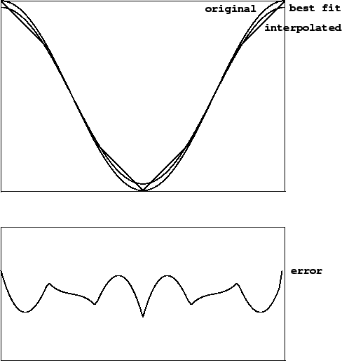
The bottom graph in the figure shows the difference between the interpolated waveform and the best-fitting sinusoid. This is a residual signal all of whose energy lies in overtones of the original sinusoid. As the number of points increases, the error decreases in magnitude. Since the error is the difference between a sinusoid and a sequence of approximating line segments, the magnitude of the error is roughly proportional to the square of the phase difference between each pair of points, or in other words, inversely proportional to the square of the number of points in the wavetable. Put another way, wavetable error decreases by 12 dB each time the table doubles in size. (This rule of thumb is only good for tables with 4 or more points.) <P> Four-point (cubic) interpolation works similarly. The interpolation formula is: <BR><P></P> <DIV ALIGN="CENTER"> <!-- MATH \begin{displaymath} {y_{\mathrm{INT}}}(x) = \end{displaymath} --> <IMG WIDTH="69" HEIGHT="28" BORDER="0" SRC="img254.png" ALT="\begin{displaymath} {y_{\mathrm{INT}}}(x) = \end{displaymath}"> </DIV> <BR CLEAR="ALL"> <P></P> <BR><P></P> <DIV ALIGN="CENTER"> <!-- MATH \begin{displaymath} -f (f-1)(f-2)/6 \cdot y[{x_0}-1] + (f+1)(f-1)(f-2)/2 \cdot y[{x_0}] \end{displaymath} --> <IMG WIDTH="435" HEIGHT="28" BORDER="0" SRC="img255.png" ALT="\begin{displaymath} -f (f-1)(f-2)/6 \cdot y[{x_0}-1] + (f+1)(f-1)(f-2)/2 \cdot y[{x_0}] \end{displaymath}"> </DIV> <BR CLEAR="ALL"> <P></P> <BR><P></P> <DIV ALIGN="CENTER"> <!-- MATH \begin{displaymath} - (f+1) f (f-2) / 2 \cdot y[{x_0}+1] + (f+1) f (f-1) / 6 \cdot y[{x_0}+2] \end{displaymath} --> <IMG WIDTH="422" HEIGHT="28" BORDER="0" SRC="img256.png" ALT="\begin{displaymath} - (f+1) f (f-2) / 2 \cdot y[{x_0}+1] + (f+1) f (f-1) / 6 \cdot y[{x_0}+2] \end{displaymath}"> </DIV> <BR CLEAR="ALL"> <P></P> where <IMG WIDTH="79" HEIGHT="30" ALIGN="MIDDLE" BORDER="0" SRC="img257.png" ALT="$f = x - {x_0}$"> is the fractional part of the index. For tables with 4 or more points, doubling the number of points on the table tends to improve the RMS error by 24 dB. Table 2.1 shows the calculated RMS error for sinusoids at various periods for 1, 2, and 4 point interpolation. (A slightly different quantity is measured in [<A HREF="node202.html#r-moore90">Moo90</A>, p.164]. There, the errors in amplitude and phase are also added in, yielding slightly more pessimistic results. See also [<A HREF="node202.html#r-hartmann87">Har87</A>].) <P> <BR><P></P> <DIV ALIGN="CENTER"><A NAME="2392"></A> <TABLE> <CAPTION><STRONG>Table 2.1:</STRONG> RMS error for table lookup using 1, 2, and 4 point interpolation at various table sizes.</CAPTION> <TR><TD><TABLE CELLPADDING=3 BORDER="1"> <TR><TD ALIGN="RIGHT">period</TD> <TD ALIGN="CENTER" COLSPAN=3>interpolation points</TD> </TR> <TR><TD ALIGN="RIGHT"> </TD> <TD ALIGN="RIGHT">1</TD> <TD ALIGN="RIGHT">2</TD> <TD ALIGN="RIGHT">4</TD> </TR> <TR><TD ALIGN="RIGHT">2</TD> <TD ALIGN="RIGHT">-1.2</TD> <TD ALIGN="RIGHT">-17.1</TD> <TD ALIGN="RIGHT">-20.2</TD> </TR> <TR><TD ALIGN="RIGHT">3</TD> <TD ALIGN="RIGHT">-2.0</TD> <TD ALIGN="RIGHT">-11.9</TD> <TD ALIGN="RIGHT">-15.5</TD> </TR> <TR><TD ALIGN="RIGHT">4</TD> <TD ALIGN="RIGHT">-4.2</TD> <TD ALIGN="RIGHT">-17.1</TD> <TD ALIGN="RIGHT">-24.8</TD> </TR> <TR><TD ALIGN="RIGHT">8</TD> <TD ALIGN="RIGHT">-10.0</TD> <TD ALIGN="RIGHT">-29.6</TD> <TD ALIGN="RIGHT">-48.4</TD> </TR> <TR><TD ALIGN="RIGHT">16</TD> <TD ALIGN="RIGHT">-15.9</TD> <TD ALIGN="RIGHT">-41.8</TD> <TD ALIGN="RIGHT">-72.5</TD> </TR> <TR><TD ALIGN="RIGHT">32</TD> <TD ALIGN="RIGHT">-21.9</TD> <TD ALIGN="RIGHT">-53.8</TD> <TD ALIGN="RIGHT">-96.5</TD> </TR> <TR><TD ALIGN="RIGHT">64</TD> <TD ALIGN="RIGHT">-27.9</TD> <TD ALIGN="RIGHT">-65.9</TD> <TD ALIGN="RIGHT">-120.6</TD> </TR> <TR><TD ALIGN="RIGHT">128</TD> <TD ALIGN="RIGHT">-34.0</TD> <TD ALIGN="RIGHT">-77.9</TD> <TD ALIGN="RIGHT">-144.7</TD> </TR> </TABLE> <A NAME="tab02.1"></A></TD></TR> </TABLE> </DIV><P></P> <BR> <P> The allowable input domain for table lookup depends on the number of points of interpolation. In general, when using <IMG WIDTH="12" HEIGHT="14" ALIGN="BOTTOM" BORDER="0" SRC="img58.png" ALT="$k$">-point interpolation into a table with <IMG WIDTH="18" HEIGHT="14" ALIGN="BOTTOM" BORDER="0" SRC="img3.png" ALT="$N$"> points, the input may range over an interval of <IMG WIDTH="73" HEIGHT="30" ALIGN="MIDDLE" BORDER="0" SRC="img258.png" ALT="$N + 1 - k$"> points. If <IMG WIDTH="41" HEIGHT="14" ALIGN="BOTTOM" BORDER="0" SRC="img259.png" ALT="$k=1$"> (i.e., no interpolation at all), the domain is from <IMG WIDTH="11" HEIGHT="13" ALIGN="BOTTOM" BORDER="0" SRC="img179.png" ALT="$0$"> to <IMG WIDTH="18" HEIGHT="14" ALIGN="BOTTOM" BORDER="0" SRC="img3.png" ALT="$N$"> (including the endpoint at <IMG WIDTH="11" HEIGHT="13" ALIGN="BOTTOM" BORDER="0" SRC="img179.png" ALT="$0$"> but excluding the one at <IMG WIDTH="18" HEIGHT="14" ALIGN="BOTTOM" BORDER="0" SRC="img3.png" ALT="$N$">) assuming input values are truncated (as is done for non-interpolated table lookup in Pd). The domain is from -<IMG WIDTH="27" HEIGHT="32" ALIGN="MIDDLE" BORDER="0" SRC="img98.png" ALT="$1/2$"> to <IMG WIDTH="61" HEIGHT="32" ALIGN="MIDDLE" BORDER="0" SRC="img260.png" ALT="$N-1/2$"> if, instead, we round the input to the nearest integer instead of interpolating. In either case, the domain stretches over a length of <IMG WIDTH="18" HEIGHT="14" ALIGN="BOTTOM" BORDER="0" SRC="img3.png" ALT="$N$"> points. <P> For two-point interpolation, the input must lie between the first and last points, that is, between <IMG WIDTH="11" HEIGHT="13" ALIGN="BOTTOM" BORDER="0" SRC="img179.png" ALT="$0$"> and <IMG WIDTH="45" HEIGHT="30" ALIGN="MIDDLE" BORDER="0" SRC="img171.png" ALT="$N-1$">. So the <IMG WIDTH="18" HEIGHT="14" ALIGN="BOTTOM" BORDER="0" SRC="img3.png" ALT="$N$"> points suffice to define the function over a domain of length <IMG WIDTH="45" HEIGHT="30" ALIGN="MIDDLE" BORDER="0" SRC="img171.png" ALT="$N-1$">. For four-point interpolation, we cannot get values for inputs between 0 and 1 (not having the required two points to the left of the input) and neither can we for the space between the last two points (<IMG WIDTH="45" HEIGHT="30" ALIGN="MIDDLE" BORDER="0" SRC="img261.png" ALT="$N-2$"> and <IMG WIDTH="45" HEIGHT="30" ALIGN="MIDDLE" BORDER="0" SRC="img171.png" ALT="$N-1$">). So in this case the domain reaches from <IMG WIDTH="11" HEIGHT="13" ALIGN="BOTTOM" BORDER="0" SRC="img262.png" ALT="$1$"> to <IMG WIDTH="45" HEIGHT="30" ALIGN="MIDDLE" BORDER="0" SRC="img261.png" ALT="$N-2$"> and has length <IMG WIDTH="45" HEIGHT="30" ALIGN="MIDDLE" BORDER="0" SRC="img263.png" ALT="$N-3$">. <P> Periodic waveforms stored in wavetables require special treatment at the ends of the table. For example, suppose we wish to store a pure sinusoid of length <IMG WIDTH="18" HEIGHT="14" ALIGN="BOTTOM" BORDER="0" SRC="img3.png" ALT="$N$">. For non-interpolating table lookup, it suffices to set, for example, <BR><P></P> <DIV ALIGN="CENTER"> <!-- MATH \begin{displaymath} x[n] = \cos(2 \pi n / N) ,\, n = 0, \ldots, N-1 \end{displaymath} --> <IMG WIDTH="255" HEIGHT="28" BORDER="0" SRC="img264.png" ALT="\begin{displaymath} x[n] = \cos(2 \pi n / N) ,\, n = 0, \ldots, N-1 \end{displaymath}"> </DIV> <BR CLEAR="ALL"> <P></P> For two-point interpolation, we need <IMG WIDTH="45" HEIGHT="30" ALIGN="MIDDLE" BORDER="0" SRC="img265.png" ALT="$N+1$"> points: <BR><P></P> <DIV ALIGN="CENTER"> <!-- MATH \begin{displaymath} x[n] = \cos(2 \pi n / N) ,\, n = 0, \ldots, N \end{displaymath} --> <IMG WIDTH="228" HEIGHT="28" BORDER="0" SRC="img266.png" ALT="\begin{displaymath} x[n] = \cos(2 \pi n / N) ,\, n = 0, \ldots, N \end{displaymath}"> </DIV> <BR CLEAR="ALL"> <P></P> In other words, we must repeat the first (<IMG WIDTH="42" HEIGHT="13" ALIGN="BOTTOM" BORDER="0" SRC="img79.png" ALT="$n=0$">) point at the end, so that the last segment from <IMG WIDTH="45" HEIGHT="30" ALIGN="MIDDLE" BORDER="0" SRC="img171.png" ALT="$N-1$"> to <IMG WIDTH="18" HEIGHT="14" ALIGN="BOTTOM" BORDER="0" SRC="img3.png" ALT="$N$"> reaches back to the beginning value. <P> For four-point interpolation, the cycle must be adjusted to start at the point <IMG WIDTH="42" HEIGHT="13" ALIGN="BOTTOM" BORDER="0" SRC="img267.png" ALT="$n=1$">, since we can't get properly interpolated values out for inputs less than one. If, then, one cycle of the wavetable is arranged from <IMG WIDTH="11" HEIGHT="13" ALIGN="BOTTOM" BORDER="0" SRC="img262.png" ALT="$1$"> to <IMG WIDTH="18" HEIGHT="14" ALIGN="BOTTOM" BORDER="0" SRC="img3.png" ALT="$N$">, we must supply extra points for <IMG WIDTH="11" HEIGHT="13" ALIGN="BOTTOM" BORDER="0" SRC="img179.png" ALT="$0$"> (copied from <IMG WIDTH="18" HEIGHT="14" ALIGN="BOTTOM" BORDER="0" SRC="img3.png" ALT="$N$">), and also <IMG WIDTH="45" HEIGHT="30" ALIGN="MIDDLE" BORDER="0" SRC="img265.png" ALT="$N+1$"> and <IMG WIDTH="45" HEIGHT="30" ALIGN="MIDDLE" BORDER="0" SRC="img268.png" ALT="$N+2$">, copied from <IMG WIDTH="11" HEIGHT="13" ALIGN="BOTTOM" BORDER="0" SRC="img262.png" ALT="$1$"> and <IMG WIDTH="11" HEIGHT="13" ALIGN="BOTTOM" BORDER="0" SRC="img269.png" ALT="$2$">, to make a table of length <IMG WIDTH="45" HEIGHT="30" ALIGN="MIDDLE" BORDER="0" SRC="img270.png" ALT="$N+3$">. For the same sinusoid as above, the table should contain: <BR><P></P> <DIV ALIGN="CENTER"> <!-- MATH \begin{displaymath} x[n] = \cos(2 \pi (n-1) / N) ,\, n = 0, \ldots, N+2 \end{displaymath} --> <IMG WIDTH="294" HEIGHT="28" BORDER="0" SRC="img271.png" ALT="\begin{displaymath} x[n] = \cos(2 \pi (n-1) / N) ,\, n = 0, \ldots, N+2 \end{displaymath}"> </DIV> <BR CLEAR="ALL"> <P></P> <P> <HR> <!--Navigation Panel--> <A NAME="tex2html1002" HREF="node32.html"> <IMG WIDTH="37" HEIGHT="24" ALIGN="BOTTOM" BORDER="0" ALT="next" SRC="file:/usr/local/share/lib/latex2html/icons/next.png"></A> <A NAME="tex2html996" HREF="node26.html"> <IMG WIDTH="26" HEIGHT="24" ALIGN="BOTTOM" BORDER="0" ALT="up" SRC="file:/usr/local/share/lib/latex2html/icons/up.png"></A> <A NAME="tex2html990" HREF="node30.html"> <IMG WIDTH="63" HEIGHT="24" ALIGN="BOTTOM" BORDER="0" ALT="previous" SRC="file:/usr/local/share/lib/latex2html/icons/prev.png"></A> <A NAME="tex2html998" HREF="node4.html"> <IMG WIDTH="65" HEIGHT="24" ALIGN="BOTTOM" BORDER="0" ALT="contents" SRC="file:/usr/local/share/lib/latex2html/icons/contents.png"></A> <A NAME="tex2html1000" HREF="node201.html"> <IMG WIDTH="43" HEIGHT="24" ALIGN="BOTTOM" BORDER="0" ALT="index" SRC="file:/usr/local/share/lib/latex2html/icons/index.png"></A> <BR> <B> Next:</B> <A NAME="tex2html1003" HREF="node32.html">Examples</A> <B> Up:</B> <A NAME="tex2html997" HREF="node26.html">Wavetables and samplers</A> <B> Previous:</B> <A NAME="tex2html991" HREF="node30.html">Timbre stretching</A> <B> <A NAME="tex2html999" HREF="node4.html">Contents</A></B> <B> <A NAME="tex2html1001" HREF="node201.html">Index</A></B> <!--End of Navigation Panel--> <ADDRESS> Miller Puckette 2006-12-30 </ADDRESS> </BODY> </HTML>