<!DOCTYPE html> <!--Converted with LaTeX2HTML 2002-2-1 (1.71) original version by: Nikos Drakos, CBLU, University of Leeds * revised and updated by: Marcus Hennecke, Ross Moore, Herb Swan * with significant contributions from: Jens Lippmann, Marek Rouchal, Martin Wilck and others --> <HTML> <HEAD> <meta name="viewport" content="width=device-width, initial-scale=1.0"> <TITLE>Stretching the unit circle with rational functions</TITLE> <META NAME="description" CONTENT="Stretching the unit circle with rational functions"> <META NAME="keywords" CONTENT="book"> <META NAME="resource-type" CONTENT="document"> <META NAME="distribution" CONTENT="global"> <META NAME="Generator" CONTENT="LaTeX2HTML v2002-2-1"> <META HTTP-EQUIV="Content-Style-Type" CONTENT="text/css"> <LINK REL="STYLESHEET" HREF="book.css"> <LINK REL="next" HREF="node147.html"> <LINK REL="previous" HREF="node145.html"> <LINK REL="up" HREF="node139.html"> <LINK REL="next" HREF="node147.html"> </HEAD> <BODY > <!--Navigation Panel--> <A ID="tex2html2758" HREF="node147.html"> <IMG WIDTH="37" HEIGHT="24" ALIGN="BOTTOM" BORDER="0" ALT="next" SRC="next.png"></A> <A ID="tex2html2752" HREF="node139.html"> <IMG WIDTH="26" HEIGHT="24" ALIGN="BOTTOM" BORDER="0" ALT="up" SRC="up.png"></A> <A ID="tex2html2746" HREF="node145.html"> <IMG WIDTH="63" HEIGHT="24" ALIGN="BOTTOM" BORDER="0" ALT="previous" SRC="prev.png"></A> <A ID="tex2html2754" HREF="node4.html"> <IMG WIDTH="65" HEIGHT="24" ALIGN="BOTTOM" BORDER="0" ALT="contents" SRC="contents.png"></A> <A ID="tex2html2756" HREF="node201.html"> <IMG WIDTH="43" HEIGHT="24" ALIGN="BOTTOM" BORDER="0" ALT="index" SRC="index.png"></A> <BR> <B> Next:</B> <A ID="tex2html2759" HREF="node147.html">Butterworth band-pass filter</A> <B> Up:</B> <A ID="tex2html2753" HREF="node139.html">Designing filters</A> <B> Previous:</B> <A ID="tex2html2747" HREF="node145.html">Butterworth filters</A> <B> <A ID="tex2html2755" HREF="node4.html">Contents</A></B> <B> <A ID="tex2html2757" HREF="node201.html">Index</A></B> <BR> <BR> <!--End of Navigation Panel--> <H2><A ID="SECTION001237000000000000000"> Stretching the unit circle with rational functions</A> </H2> <P> In Section <A HREF="node143.html#sect8.twopolebandpass">8.3.4</A> we saw a simple way to turn a low-pass filter into a band-pass one. It is tempting to apply the same method to turn our Butterworth low-pass filter into a higher-quality band-pass filter; but if we wish to preserve the high quality of the Butterworth filter we must be more careful than before in the design of the transformation used. In this section we will prepare the way to making the Butterworth band-pass filter by introducing a class of rational transformations of the complex plane which preserve the unit circle. <P> This discussion is adapted from [<A HREF="node202.html#r-parks87">PB87</A>], pp. 201-206 (I'm grateful to Julius Smith for this pointer). There the transformation is carried out in continuous time, but here we have adapted the method to operate in discrete time, in order to make the discussion self-contained. <P> The idea is to start with any filter with a transfer function as before: <BR><P></P> <DIV ALIGN="CENTER"> <!-- MATH \begin{displaymath} H(Z) = { { (1 - {Q_1}{Z^{-1}}) \cdots (1 - {Q_j}{Z^{-1}}) } \over { (1 - {P_1}{Z^{-1}}) \cdots (1 - {P_k}{Z^{-1}}) } } \end{displaymath} --> <IMG WIDTH="263" HEIGHT="45" BORDER="0" SRC="img889.png" ALT="\begin{displaymath} H(Z) = { { (1 - {Q_1}{Z^{-1}}) \cdots (1 - {Q_j}{Z^{-1}}) } \over { (1 - {P_1}{Z^{-1}}) \cdots (1 - {P_k}{Z^{-1}}) } } \end{displaymath}"> </DIV> <BR CLEAR="ALL"> <P></P> whose frequency response (the gain at a frequency <IMG WIDTH="14" HEIGHT="13" ALIGN="BOTTOM" BORDER="0" SRC="img27.png" ALT="$\omega $">) is given by: <BR><P></P> <DIV ALIGN="CENTER"> <!-- MATH \begin{displaymath} | H(\cos(\omega) + i \sin(\omega)) | \end{displaymath} --> <IMG WIDTH="146" HEIGHT="28" BORDER="0" SRC="img938.png" ALT="\begin{displaymath} \vert H(\cos(\omega) + i \sin(\omega)) \vert \end{displaymath}"> </DIV> <BR CLEAR="ALL"> <P></P> <P> Now suppose we can find a rational function, <IMG WIDTH="40" HEIGHT="32" ALIGN="MIDDLE" BORDER="0" SRC="img939.png" ALT="$R(Z)$">, which distorts the unit circle in some desirable way. For <IMG WIDTH="15" HEIGHT="14" ALIGN="BOTTOM" BORDER="0" SRC="img36.png" ALT="$R$"> to be a rational function means that it can be written as a quotient of two polynomials (for example, the transfer function <IMG WIDTH="18" HEIGHT="14" ALIGN="BOTTOM" BORDER="0" SRC="img25.png" ALT="$H$"> is a rational function). That <IMG WIDTH="15" HEIGHT="14" ALIGN="BOTTOM" BORDER="0" SRC="img36.png" ALT="$R$"> sends points on the unit circle to other points on the unit circle is just the condition that <IMG WIDTH="78" HEIGHT="32" ALIGN="MIDDLE" BORDER="0" SRC="img940.png" ALT="$\vert R(Z)\vert = 1$"> whenever <IMG WIDTH="44" HEIGHT="14" ALIGN="BOTTOM" BORDER="0" SRC="img941.png" ALT="$Z=1$">. It can easily be checked that any function of the form <BR><P></P> <DIV ALIGN="CENTER"> <!-- MATH \begin{displaymath} R(Z) = U \cdot {{ {A_n}{Z^n} + {A_{n-1}}{Z^{n-1}} + \cdots + {A_0} } \over { \overline{A_0}{Z^n} + \overline{A_1}{Z^{n-1}} + \cdots + \overline{A_n} }} \end{displaymath} --> <IMG WIDTH="295" HEIGHT="45" BORDER="0" SRC="img942.png" ALT="\begin{displaymath} R(Z) = U \cdot {{ {A_n}{Z^n} + {A_{n-1}}{Z^{n-1}} + \cdot... ...}{Z^n} + \overline{A_1}{Z^{n-1}} + \cdots + \overline{A_n} }} \end{displaymath}"> </DIV> <BR CLEAR="ALL"> <P></P> (where <IMG WIDTH="54" HEIGHT="32" ALIGN="MIDDLE" BORDER="0" SRC="img943.png" ALT="$\vert U\vert=1$">) has this property. The same reasoning as in Section <A HREF="node134.html#sect8.secondform">8.2.2</A> confirms that <IMG WIDTH="78" HEIGHT="32" ALIGN="MIDDLE" BORDER="0" SRC="img940.png" ALT="$\vert R(Z)\vert = 1$"> whenever <IMG WIDTH="44" HEIGHT="14" ALIGN="BOTTOM" BORDER="0" SRC="img941.png" ALT="$Z=1$">. <P> Once we have a suitable rational function <IMG WIDTH="15" HEIGHT="14" ALIGN="BOTTOM" BORDER="0" SRC="img36.png" ALT="$R$">, we can simply compose it with the original transfer function <IMG WIDTH="18" HEIGHT="14" ALIGN="BOTTOM" BORDER="0" SRC="img25.png" ALT="$H$"> to fabricate a new rational function, <BR><P></P> <DIV ALIGN="CENTER"> <!-- MATH \begin{displaymath} J(Z) = H(R(Z)) \end{displaymath} --> <IMG WIDTH="117" HEIGHT="28" BORDER="0" SRC="img944.png" ALT="\begin{displaymath} J(Z) = H(R(Z)) \end{displaymath}"> </DIV> <BR CLEAR="ALL"> <P></P> The gain of the new filter <IMG WIDTH="13" HEIGHT="14" ALIGN="BOTTOM" BORDER="0" SRC="img945.png" ALT="$J$"> at the frequency <IMG WIDTH="14" HEIGHT="13" ALIGN="BOTTOM" BORDER="0" SRC="img27.png" ALT="$\omega $"> is then equal to that of <IMG WIDTH="18" HEIGHT="14" ALIGN="BOTTOM" BORDER="0" SRC="img25.png" ALT="$H$"> at a different frequency <IMG WIDTH="13" HEIGHT="30" ALIGN="MIDDLE" BORDER="0" SRC="img77.png" ALT="$\phi$">, chosen so that: <BR><P></P> <DIV ALIGN="CENTER"> <!-- MATH \begin{displaymath} \cos(\phi) + i \sin(\phi) = R(\cos(\omega) + i \sin(\omega)) \end{displaymath} --> <IMG WIDTH="270" HEIGHT="28" BORDER="0" SRC="img946.png" ALT="\begin{displaymath} \cos(\phi) + i \sin(\phi) = R(\cos(\omega) + i \sin(\omega)) \end{displaymath}"> </DIV> <BR CLEAR="ALL"> <P></P> The function <IMG WIDTH="15" HEIGHT="14" ALIGN="BOTTOM" BORDER="0" SRC="img36.png" ALT="$R$"> moves points around on the unit circle; <IMG WIDTH="13" HEIGHT="14" ALIGN="BOTTOM" BORDER="0" SRC="img945.png" ALT="$J$"> at any point equals <IMG WIDTH="18" HEIGHT="14" ALIGN="BOTTOM" BORDER="0" SRC="img25.png" ALT="$H$"> on the point <IMG WIDTH="15" HEIGHT="14" ALIGN="BOTTOM" BORDER="0" SRC="img36.png" ALT="$R$"> moves it to. <P> 
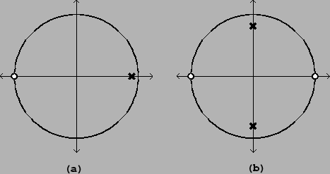
For example, suppose we start with a one-zero, one-pole low-pass filter: <BR><P></P> <DIV ALIGN="CENTER"> <!-- MATH \begin{displaymath} H(Z) = {{ 1 + {Z^{-1}} } \over { 1 - g{Z^{-1}} }} \end{displaymath} --> <IMG WIDTH="127" HEIGHT="44" BORDER="0" SRC="img947.png" ALT="\begin{displaymath} H(Z) = {{ 1 + {Z^{-1}} } \over { 1 - g{Z^{-1}} }} \end{displaymath}"> </DIV> <BR CLEAR="ALL"> <P></P> and apply the function <BR><P></P> <DIV ALIGN="CENTER"> <!-- MATH \begin{displaymath} R(Z) = -{Z^2} = - {{ 1 \cdot {Z^2} + 0 \cdot Z + 0 } \over { 0 \cdot {Z^2} + 0 \cdot Z + 1 }} \end{displaymath} --> <IMG WIDTH="242" HEIGHT="42" BORDER="0" SRC="img948.png" ALT="\begin{displaymath} R(Z) = -{Z^2} = - {{ 1 \cdot {Z^2} + 0 \cdot Z + 0 } \over { 0 \cdot {Z^2} + 0 \cdot Z + 1 }} \end{displaymath}"> </DIV> <BR CLEAR="ALL"> <P></P> Geometrically, this choice of <IMG WIDTH="15" HEIGHT="14" ALIGN="BOTTOM" BORDER="0" SRC="img36.png" ALT="$R$"> stretches the unit circle uniformly to twice its circumference and wraps it around itself twice. The points <IMG WIDTH="11" HEIGHT="13" ALIGN="BOTTOM" BORDER="0" SRC="img262.png" ALT="$1$"> and <IMG WIDTH="23" HEIGHT="29" ALIGN="MIDDLE" BORDER="0" SRC="img401.png" ALT="$-1$"> are both sent to the point <IMG WIDTH="23" HEIGHT="29" ALIGN="MIDDLE" BORDER="0" SRC="img401.png" ALT="$-1$">, and the points <IMG WIDTH="9" HEIGHT="14" ALIGN="BOTTOM" BORDER="0" SRC="img646.png" ALT="$i$"> and <IMG WIDTH="21" HEIGHT="29" ALIGN="MIDDLE" BORDER="0" SRC="img949.png" ALT="$-i$"> are sent to the point <IMG WIDTH="11" HEIGHT="13" ALIGN="BOTTOM" BORDER="0" SRC="img262.png" ALT="$1$">. The resulting transfer function is <BR><P></P> <DIV ALIGN="CENTER"> <!-- MATH \begin{displaymath} J(Z) = {{ 1 - {Z^{-2}} } \over { 1 + g{Z^{-2}} }} = {{ (1 - {Z^{-1}})(1 + {Z^{-1}}) } \over { (1 - i\sqrt{g} {Z^{-1}})(1 + i\sqrt{g} {Z^{-1}}) }} \end{displaymath} --> <IMG WIDTH="339" HEIGHT="46" BORDER="0" SRC="img950.png" ALT="\begin{displaymath} J(Z) = {{ 1 - {Z^{-2}} } \over { 1 + g{Z^{-2}} }} = ... ... \over { (1 - i\sqrt{g} {Z^{-1}})(1 + i\sqrt{g} {Z^{-1}}) }} \end{displaymath}"> </DIV> <BR CLEAR="ALL"> <P></P> The pole-zero plots of <IMG WIDTH="18" HEIGHT="14" ALIGN="BOTTOM" BORDER="0" SRC="img25.png" ALT="$H$"> and <IMG WIDTH="13" HEIGHT="14" ALIGN="BOTTOM" BORDER="0" SRC="img945.png" ALT="$J$"> are shown in Figure <A HREF="#fig08.19">8.19</A>. From a low-pass filter we ended up with a band-pass filter. The points <IMG WIDTH="9" HEIGHT="14" ALIGN="BOTTOM" BORDER="0" SRC="img646.png" ALT="$i$"> and <IMG WIDTH="21" HEIGHT="29" ALIGN="MIDDLE" BORDER="0" SRC="img949.png" ALT="$-i$"> which <IMG WIDTH="15" HEIGHT="14" ALIGN="BOTTOM" BORDER="0" SRC="img36.png" ALT="$R$"> sends to <IMG WIDTH="11" HEIGHT="13" ALIGN="BOTTOM" BORDER="0" SRC="img262.png" ALT="$1$"> (where the original filter's gain is highest) become points of highest gain for the new filter. <P> <DIV ALIGN="CENTER"><A ID="fig08.19"></A><A ID="10765"></A> <TABLE> <CAPTION ALIGN="BOTTOM"><STRONG>Figure 8.19:</STRONG> One-pole, one-zero low-pass filter: (a) pole-zero plot; (b) plot for the resulting filter after the transformation <IMG WIDTH="92" HEIGHT="34" ALIGN="MIDDLE" BORDER="0" SRC="img51.png" ALT="$R(Z) = -{Z^2}$">. The result is a band-pass filter with center frequency <IMG WIDTH="29" HEIGHT="32" ALIGN="MIDDLE" BORDER="0" SRC="img5.png" ALT="$\pi /2$">. </CAPTION> <TR><TD><IMG WIDTH="467" HEIGHT="247" BORDER="0" SRC="img951.png" ALT="\begin{figure}\psfig{file=figs/fig08.19.ps}\end{figure}"></TD></TR> </TABLE> </DIV> <P> <HR> <!--Navigation Panel--> <A ID="tex2html2758" HREF="node147.html"> <IMG WIDTH="37" HEIGHT="24" ALIGN="BOTTOM" BORDER="0" ALT="next" SRC="next.png"></A> <A ID="tex2html2752" HREF="node139.html"> <IMG WIDTH="26" HEIGHT="24" ALIGN="BOTTOM" BORDER="0" ALT="up" SRC="up.png"></A> <A ID="tex2html2746" HREF="node145.html"> <IMG WIDTH="63" HEIGHT="24" ALIGN="BOTTOM" BORDER="0" ALT="previous" SRC="prev.png"></A> <A ID="tex2html2754" HREF="node4.html"> <IMG WIDTH="65" HEIGHT="24" ALIGN="BOTTOM" BORDER="0" ALT="contents" SRC="contents.png"></A> <A ID="tex2html2756" HREF="node201.html"> <IMG WIDTH="43" HEIGHT="24" ALIGN="BOTTOM" BORDER="0" ALT="index" SRC="index.png"></A> <BR> <B> Next:</B> <A ID="tex2html2759" HREF="node147.html">Butterworth band-pass filter</A> <B> Up:</B> <A ID="tex2html2753" HREF="node139.html">Designing filters</A> <B> Previous:</B> <A ID="tex2html2747" HREF="node145.html">Butterworth filters</A> <B> <A ID="tex2html2755" HREF="node4.html">Contents</A></B> <B> <A ID="tex2html2757" HREF="node201.html">Index</A></B> <!--End of Navigation Panel--> <ADDRESS> Miller Puckette 2006-12-30 </ADDRESS> </BODY> </HTML>