<!DOCTYPE html> <!--Converted with LaTeX2HTML 2002-2-1 (1.71) original version by: Nikos Drakos, CBLU, University of Leeds * revised and updated by: Marcus Hennecke, Ross Moore, Herb Swan * with significant contributions from: Jens Lippmann, Marek Rouchal, Martin Wilck and others --> <HTML> <HEAD> <meta name="viewport" content="width=device-width, initial-scale=1.0"> <TITLE>Control streams</TITLE> <META NAME="description" CONTENT="Control streams"> <META NAME="keywords" CONTENT="book"> <META NAME="resource-type" CONTENT="document"> <META NAME="distribution" CONTENT="global"> <META NAME="Generator" CONTENT="LaTeX2HTML v2002-2-1"> <META HTTP-EQUIV="Content-Style-Type" CONTENT="text/css"> <LINK REL="STYLESHEET" HREF="book.css"> <LINK REL="next" HREF="node44.html"> <LINK REL="previous" HREF="node42.html"> <LINK REL="up" HREF="node40.html"> <LINK REL="next" HREF="node44.html"> </HEAD> <BODY > <!--Navigation Panel--> <A NAME="tex2html1189" HREF="node44.html"> <IMG WIDTH="37" HEIGHT="24" ALIGN="BOTTOM" BORDER="0" ALT="next" SRC="next.png"></A> <A NAME="tex2html1183" HREF="node40.html"> <IMG WIDTH="26" HEIGHT="24" ALIGN="BOTTOM" BORDER="0" ALT="up" SRC="up.png"></A> <A NAME="tex2html1177" HREF="node42.html"> <IMG WIDTH="63" HEIGHT="24" ALIGN="BOTTOM" BORDER="0" ALT="previous" SRC="prev.png"></A> <A NAME="tex2html1185" HREF="node4.html"> <IMG WIDTH="65" HEIGHT="24" ALIGN="BOTTOM" BORDER="0" ALT="contents" SRC="contents.png"></A> <A NAME="tex2html1187" HREF="node201.html"> <IMG WIDTH="43" HEIGHT="24" ALIGN="BOTTOM" BORDER="0" ALT="index" SRC="index.png"></A> <BR> <B> Next:</B> <A NAME="tex2html1190" HREF="node44.html">Converting from audio signals</A> <B> Up:</B> <A NAME="tex2html1184" HREF="node40.html">Audio and control computations</A> <B> Previous:</B> <A NAME="tex2html1178" HREF="node42.html">Control</A> <B> <A NAME="tex2html1186" HREF="node4.html">Contents</A></B> <B> <A NAME="tex2html1188" HREF="node201.html">Index</A></B> <BR> <BR> <!--End of Navigation Panel--> <H1><A NAME="SECTION00730000000000000000"></A> <A NAME="sect3.controlstreams"></A> <BR> Control streams </H1> <P> Control computations may come from a variety of sources, both internal and external to the overall computation. Examples of internally engendered control computations include sequencing (in which control computations must take place at pre-determined times) or feature detection of the audio output (for instance, watching for zero crossings in a signal). Externally engendered ones may come from input devices such as MIDI controllers, the mouse and keyboard, network packets, and so on. In any case, control computations may occur at irregular intervals, unlike audio samples which correspond to a steadily ticking sample clock. <P> <DIV ALIGN="CENTER"><A NAME="fig03.03"></A><A NAME="3592"></A> <TABLE> <CAPTION ALIGN="BOTTOM"><STRONG>Figure 3.3:</STRONG> Graphical representation of a control stream as a sequence of points in time.</CAPTION> <TR><TD><IMG WIDTH="280" HEIGHT="51" BORDER="0" SRC="img314.png" ALT="\begin{figure}\psfig{file=figs/fig03.03.ps}\end{figure}"></TD></TR> </TABLE> </DIV> <P> We will need a way of describing how information flows between control and audio computations, which we will base on the notion of a <A NAME="3595"></A><I>control stream</I>. This is simply a collection of numbers--possibly empty--that appear as a result of control computations, whether regularly or irregularly spaced in logical time. The simplest possible control stream has no information other than a <A NAME="3597"></A> <I>time sequence</I>: <BR><P></P> <DIV ALIGN="CENTER"> <!-- MATH \begin{displaymath} \ldots , t[0], t[1], t[2], \ldots \end{displaymath} --> <IMG WIDTH="133" HEIGHT="28" BORDER="0" SRC="img315.png" ALT="\begin{displaymath} \ldots , t[0], t[1], t[2], \ldots \end{displaymath}"> </DIV> <BR CLEAR="ALL"> <P></P> Although the time values are best given in units of samples, their values aren't quantized; they may be arbitrary real numbers. We do require them to be sorted in nondecreasing order: <BR><P></P> <DIV ALIGN="CENTER"> <!-- MATH \begin{displaymath} \cdots \le t[0] \le t[1] \le t[2] \le \cdots \end{displaymath} --> <IMG WIDTH="186" HEIGHT="28" BORDER="0" SRC="img316.png" ALT="\begin{displaymath} \cdots \le t[0] \le t[1] \le t[2] \le \cdots \end{displaymath}"> </DIV> <BR CLEAR="ALL"> <P></P> Each item in the sequence is called an <A NAME="3599"></A><I>event</I>. <P> 
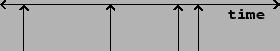
Control streams may be shown graphically as in Figure <A HREF="#fig03.03">3.3</A>. A number line shows time and a sequence of arrows points to the times associated with each event. The control stream shown has no data (it is a time sequence). If we want to show data in the control stream we will write it at the base of each arrow. <P> A <A NAME="3602"></A><I>numeric control stream</I> is one that contains one number per time point, so that it appears as a sequence of ordered pairs: <BR><P></P> <DIV ALIGN="CENTER"> <!-- MATH \begin{displaymath} \ldots , \, (t[0], x[0]), \, (t[1], x[1]), \, \ldots \end{displaymath} --> <IMG WIDTH="202" HEIGHT="28" BORDER="0" SRC="img317.png" ALT="\begin{displaymath} \ldots , \, (t[0], x[0]), \, (t[1], x[1]), \, \ldots \end{displaymath}"> </DIV> <BR CLEAR="ALL"> <P></P> where the <IMG WIDTH="27" HEIGHT="32" ALIGN="MIDDLE" BORDER="0" SRC="img318.png" ALT="$t[n]$"> are the time points and the <IMG WIDTH="31" HEIGHT="32" ALIGN="MIDDLE" BORDER="0" SRC="img80.png" ALT="$x[n]$"> are the signal's values at those times. <P> A numeric control stream is roughly analogous to a "MIDI controller", whose values change irregularly, for example when a physical control is moved by a performer. Other control stream sources may have higher possible rates of change and/or more precision. On the other hand, a time sequence might be a sequence of pedal hits, which (MIDI implementation notwithstanding) shouldn't be considered as having <I>values</I>, just <I>times</I>. <P> Numeric control streams are like audio signals in that both are just time-varying numeric values. But whereas the audio signal comes at a steady rate (and so the time values need not be specified per sample), the control stream comes unpredictably--perhaps evenly, perhaps unevenly, perhaps never. <P> Let us now look at what happens when we try to convert a numeric control stream to an audio signal. As before we'll choose a block size <IMG WIDTH="45" HEIGHT="14" ALIGN="BOTTOM" BORDER="0" SRC="img312.png" ALT="$B=4$">. We will consider as a control stream a square wave of period 5.5: <P> <BR><P></P> <DIV ALIGN="CENTER"> <!-- MATH \begin{displaymath} (2, 1), (4.75, 0), (7.5, 1), (10.25, 0), (13, 1), \ldots \end{displaymath} --> <IMG WIDTH="296" HEIGHT="28" BORDER="0" SRC="img319.png" ALT="\begin{displaymath} (2, 1), (4.75, 0), (7.5, 1), (10.25, 0), (13, 1), \ldots \end{displaymath}"> </DIV> <BR CLEAR="ALL"> <P></P> and demonstrate three ways it could be converted to an audio signal. Figure <A HREF="#fig03.04">3.4</A> (part a) shows the simplest, fast-as-possible, conversion. Each audio sample of output simply reflects the most recent value of the control signal. So samples 0 through 3 (which are computed at logical time 4 because of the block size) are 1 in value because of the point (2, 1). The next four samples are also one, because of the two points, (4.75, 0) and (7.5, 1), the most recent still has the value 1. <P> Fast-as-possible conversion is most appropriate for control streams which do not change frequently compared to the block size. Its main advantages are simplicity of computation and the fastest possible response to changes. As the figure shows, when the control stream's updates are too fast (on the order of the block size), the audio signal may not be a good likeness of the sporadic one. (If, as in this case, the control stream comes at regular intervals of time, we can use the sampling theorem to analyze the result. Here the Nyquist frequency associated with the block rate <IMG WIDTH="36" HEIGHT="32" ALIGN="MIDDLE" BORDER="0" SRC="img320.png" ALT="$R/B$"> is lower than the input square wave's frequency, and so the output is aliased to a new frequency lower than the Nyquist frequency.) <P> <DIV ALIGN="CENTER"><A NAME="fig03.04"></A><A NAME="3609"></A> <TABLE> <CAPTION ALIGN="BOTTOM"><STRONG>Figure 3.4:</STRONG> Three ways to change a control stream into an audio signal: (a) as fast as possible; (b) delayed to the nearest sample; (c) with two-point interpolation for higher delay accuracy.</CAPTION> <TR><TD><IMG WIDTH="574" HEIGHT="534" BORDER="0" SRC="img321.png" ALT="\begin{figure}\psfig{file=figs/fig03.04.ps}\end{figure}"></TD></TR> </TABLE> </DIV> <P> 
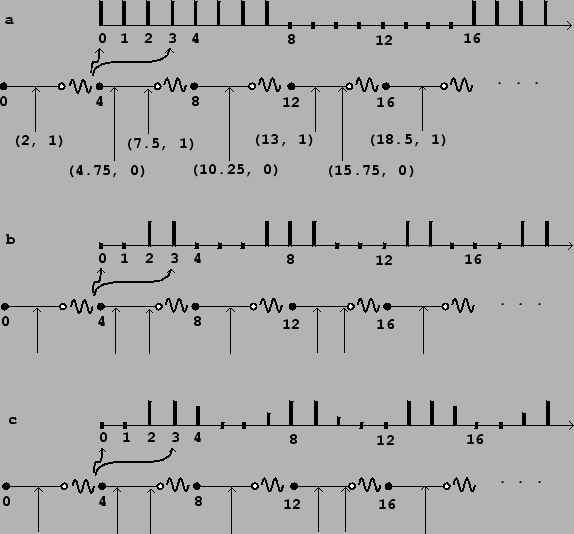
Part (b) shows the result of nearest-sample conversion. Each new value of the control stream at a time <IMG WIDTH="9" HEIGHT="13" ALIGN="BOTTOM" BORDER="0" SRC="img82.png" ALT="$t$"> affects output samples starting from index <!-- MATH $\lfloor t \rfloor$ --> <IMG WIDTH="23" HEIGHT="32" ALIGN="MIDDLE" BORDER="0" SRC="img322.png" ALT="$\lfloor t \rfloor$"> (the greatest integer not exceeding <IMG WIDTH="9" HEIGHT="13" ALIGN="BOTTOM" BORDER="0" SRC="img82.png" ALT="$t$">). This is equivalent to using fast-as-possible conversion at a block size of 1; in other words, nearest-sample conversion hides the effect of the larger block size. This is better than fast-as-possible conversion in cases where the control stream might change quickly. <P> Part (c) shows sporadic-to-audio conversion, again at the nearest sample, but now also using two-point interpolation to further increase the time accuracy. Conceptually we can describe this as follows. Suppose the value of the control stream was last equal to <IMG WIDTH="12" HEIGHT="13" ALIGN="BOTTOM" BORDER="0" SRC="img243.png" ALT="$x$">, and that the next point is <IMG WIDTH="68" HEIGHT="32" ALIGN="MIDDLE" BORDER="0" SRC="img323.png" ALT="$(n+f, y)$">, where <IMG WIDTH="13" HEIGHT="13" ALIGN="BOTTOM" BORDER="0" SRC="img75.png" ALT="$n$"> is an integer and <IMG WIDTH="13" HEIGHT="30" ALIGN="MIDDLE" BORDER="0" SRC="img112.png" ALT="$f$"> is the fractional part of the time value (so <IMG WIDTH="71" HEIGHT="30" ALIGN="MIDDLE" BORDER="0" SRC="img324.png" ALT="$0 \le f < 1$">). The first point affected in the audio output will be the sample at index <IMG WIDTH="13" HEIGHT="13" ALIGN="BOTTOM" BORDER="0" SRC="img75.png" ALT="$n$">. But instead of setting the output to <IMG WIDTH="11" HEIGHT="29" ALIGN="MIDDLE" BORDER="0" SRC="img106.png" ALT="$y$"> as before, we set it to <BR><P></P> <DIV ALIGN="CENTER"> <!-- MATH \begin{displaymath} fx + (1-f)y, \end{displaymath} --> <IMG WIDTH="99" HEIGHT="28" BORDER="0" SRC="img325.png" ALT="\begin{displaymath} fx + (1-f)y, \end{displaymath}"> </DIV> <BR CLEAR="ALL"> <P></P> in other words, to a weighted average of the previous and the new value, whose weights favor the new value more if the time of the sporadic value is earlier, closer to <IMG WIDTH="13" HEIGHT="13" ALIGN="BOTTOM" BORDER="0" SRC="img75.png" ALT="$n$">. In the example shown, the transition from 0 to 1 at time 2 gives <BR><P></P> <DIV ALIGN="CENTER"> <!-- MATH \begin{displaymath} 0 \cdot x + 1 \cdot y = 1, \end{displaymath} --> <IMG WIDTH="108" HEIGHT="27" BORDER="0" SRC="img326.png" ALT="\begin{displaymath} 0 \cdot x + 1 \cdot y = 1, \end{displaymath}"> </DIV> <BR CLEAR="ALL"> <P></P> while the transition from 1 to 0 at time 4.75 gives: <BR><P></P> <DIV ALIGN="CENTER"> <!-- MATH \begin{displaymath} 0.75 \cdot x + 0.25 \cdot y = 0.75. \end{displaymath} --> <IMG WIDTH="168" HEIGHT="27" BORDER="0" SRC="img327.png" ALT="\begin{displaymath} 0.75 \cdot x + 0.25 \cdot y = 0.75. \end{displaymath}"> </DIV> <BR CLEAR="ALL"> <P></P> This technique gives a still closer representation of the control signal (at least, the portion of it that lies below the Nyquist frequency), at the expense of more computation and slightly greater delay. <P> Numeric control streams may also be converted to audio signals using ramp functions to smooth discontinuities. This is often used when a control stream is used to control an amplitude, as described in Section <A HREF="node12.html#sect1.synth">1.5</A>. In general there are three values to specify to set a ramp function in motion: a start time and target value (specified by the control stream) and a target time, often expressed as a delay after the start time. <P> In such situations it is almost always accurate enough to adjust the start and ending times to match the first audio sample computed at a later logical time, a choice which corresponds to the fast-as-possible scenario above. Figure <A HREF="#fig03.05">3.5</A> (part a) shows the effect of ramping from 0, starting at time 3, to a value of 1 at time 9, immediately starting back toward 0 at time 15, with block size <IMG WIDTH="45" HEIGHT="14" ALIGN="BOTTOM" BORDER="0" SRC="img312.png" ALT="$B=4$">. The times 3, 9, and 15 are truncated to 0, 8, and 12, respectively. <P> <DIV ALIGN="CENTER"><A NAME="fig03.05"></A><A NAME="3616"></A> <TABLE> <CAPTION ALIGN="BOTTOM"><STRONG>Figure 3.5:</STRONG> Line segment smoothing of numeric control streams: (a) aligned to block boundaries; (b) aligned to nearest sample.</CAPTION> <TR><TD><IMG WIDTH="342" HEIGHT="196" BORDER="0" SRC="img328.png" ALT="\begin{figure}\psfig{file=figs/fig03.05.ps}\end{figure}"></TD></TR> </TABLE> </DIV> <P> 
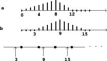
In real situations the block size might be on the order of a millisecond, and adjusting ramp endpoints to block boundaries works fine for controlling amplitudes; reaching a target a fraction of a millisecond early or late rarely makes an audible difference. However, other uses of ramps are more sensitive to time quantization of endpoints. For example, if we wish to do something repetitively every few milliseconds, the variation in segment lengths will make for an audible aperiodicity. <P> For situations such as these, we can improve the ramp generation algorithm to start and stop at arbitrary samples, as shown in Figure <A HREF="#fig03.05">3.5</A> (part b), for example. Here the endpoints of the line segments line up exactly with the requested samples 3, 9, and 15. We can go even further and adjust for fractional samples, making the line segments touch the values 0 and 1 at exactly specifiable points on a number line. <P> For example, suppose we want to repeat a recorded sound out of a wavetable 100 times per second, every 441 samples at the usual sample rate. Rounding errors due to blocking at 64-sample boundaries could detune the playback by as much as a whole tone in pitch; and even rounding to one-sample boundaries could introduce variations up to about 0.2%, or three cents. This situation would call for sub-sample accuracy in sporadic-to-audio conversion. <P> <HR> <!--Navigation Panel--> <A NAME="tex2html1189" HREF="node44.html"> <IMG WIDTH="37" HEIGHT="24" ALIGN="BOTTOM" BORDER="0" ALT="next" SRC="next.png"></A> <A NAME="tex2html1183" HREF="node40.html"> <IMG WIDTH="26" HEIGHT="24" ALIGN="BOTTOM" BORDER="0" ALT="up" SRC="up.png"></A> <A NAME="tex2html1177" HREF="node42.html"> <IMG WIDTH="63" HEIGHT="24" ALIGN="BOTTOM" BORDER="0" ALT="previous" SRC="prev.png"></A> <A NAME="tex2html1185" HREF="node4.html"> <IMG WIDTH="65" HEIGHT="24" ALIGN="BOTTOM" BORDER="0" ALT="contents" SRC="contents.png"></A> <A NAME="tex2html1187" HREF="node201.html"> <IMG WIDTH="43" HEIGHT="24" ALIGN="BOTTOM" BORDER="0" ALT="index" SRC="index.png"></A> <BR> <B> Next:</B> <A NAME="tex2html1190" HREF="node44.html">Converting from audio signals</A> <B> Up:</B> <A NAME="tex2html1184" HREF="node40.html">Audio and control computations</A> <B> Previous:</B> <A NAME="tex2html1178" HREF="node42.html">Control</A> <B> <A NAME="tex2html1186" HREF="node4.html">Contents</A></B> <B> <A NAME="tex2html1188" HREF="node201.html">Index</A></B> <!--End of Navigation Panel--> <ADDRESS> Miller Puckette 2006-12-30 </ADDRESS> </BODY> </HTML>